Deep L-layer Neural Network from Scratch in Python

In the previous article, we saw Logistic Regression with Gradient Descent and also started with Shallow Neural Network. But in real-world applications, shallow networks may under-fit data. You can check this article here.

Deep L-layer Neural Network

As shown below image, the first network (actually not network) is one neuron or logistic regression unit or perceptron. \(2^{nd}\) and \(3^{rd}\) are also considered as shallow. We don't have any predefined boundary which can say What depth of network required to become deep network?. We can say the last \(4^{th}\) network may be deep.

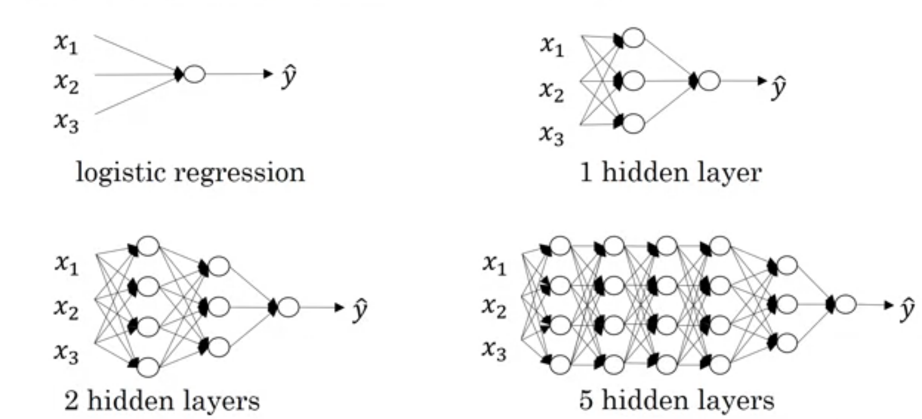
In previous article, We saw \(n^{[l]}\) is number of neurons in \(l^{th}\) layer. We will implement \(4^{th}\) neural network in the above image in this article.

Forward Propagation

Output from \(l^{th}\) layer is the sum of the weighted sum of the output of the previous layer and bias. We saw this in the previous article. Now generalize this.

\[
\begin{align*}
Z^{[l]} &= W^{[l]}.a^{[l-1]} + b^{[l]} \\
a^{[l]} &= g^{[l]}{(Z^{[l]})}
\end{align*}
\]

In above equations, \(g^{[l]}\) means activation function used in that particular layer. \(l \in \mathbb{R}^{[1,L]}\) and \(L\) means total number of layers excluding input. When \(l = 1\) then \({a^{[l-1]} = a^{[0]} = X}\)

Let's initialize weights and biases. We will use units (python list) to store units in each layer. units[0] will be input size \(n_x\). We will use a dictionary so that no need to use different variable names.

# import required libraries
import numpy as np

# create some data
m = 2  # no of samples
X = np.random.rand(3,m)
Y = np.random.rand(1,m)
alpha = 0.01 # learning rate

# units in each layer
# first number (3) is input dimension
units = [3, 4, 4, 4, 4, 3, 1]

# Total layers
L = len(units) - 1

# parameter dictionary
parameters = dict()

for layer in range(1, L+1):
    parameters['W' + str(layer)] = np.random.rand(units[layer],units[layer-1])
    parameters['b' + str(layer)] = np.zeros((units[layer],1))

Let's find predicted output using the above generic equations.

cache = dict()
cache['a0'] = X

for layer in range(1, L+1):
    cache['Z' + str(layer)] = np.dot(parameters['W' + str(layer)],cache['a' + str(layer-1)]) + parameters['b' + str(layer)]
    cache['a' + str(layer)] = sigmoid(cache['Z' + str(layer)])

cache['a' + str(L)] will be the predicted output. We completed the forward pass of the neural network. Now the important part i.e. backpropagation for updating learnable parameters.

Backward Pass

As we want generic backpropagation steps, we need to define some notations

\(dZ^{[l]}\) : error in cost function with respect to \(Z^{[l]}\)
\(da^{[l]}\) : error in cost function with respect to \(a^{[l]}\)
\(dW^{[l]}\) : error in cost function with respect to \(W^{[l]}\)
\(db^{[l]}\) : error in cost function with respect to \(b^{[l]}\)
\(g'^{[l]}(Z^{[l]})\) : derivative of activation function used in \(l^{th}\) layer i.e. \(g^{[l]}(Z^{l})\)

For backword pass, we will take some equations from our previous article. I am pasting these equations down without any proof. If you want to check proof, visit previous article.

\[ \begin{align*} \frac{\partial{J}( W,b )}{\partial{Z}} &= (\frac{1}{m})(a-y) \\ dZ^{[L]} &= (\frac{1}{m})(a^{[L]}-y) \end{align*} \]

In above equation, \(\frac{\partial{J}( W,b )}{\partial{Z}}\) means \(dZ^{[L]}\). Now to backpropagate error to previous layers we will copy-paste following equations from previous article.

\[ \begin{align*} \frac{\partial{J}(W,b)}{\partial{Z^{[1]}}} &= (W^{[2]T} . \frac{\partial{J}(W,b)}{\partial{Z^{[2]}}}) * \sigma'{(Z^{[1]})}\\ \frac{\partial{J}(W,b)}{\partial{Z^{[l]}}} &= (W^{[l+1]T} . \frac{\partial{J}(W,b)}{\partial{Z^{[l+1]}}}) * \sigma'{(Z^{[l]})}\\ dZ^{[l]} &= (W^{[l+1]T} . dZ^{[l+1]}) * g'^{[l]}(Z^{[l]}) \end{align*} \]

Now we need equations for updating weights and bias. What do you think... Let's copy them also

\[ \begin{align*} \frac{\partial{J}(W,b)}{\partial{W^{[1]}}} &= \frac{\partial{J}(W,b)}{\partial{Z^{[1]}}} .X^{T}\\ dW^{[l]} &= dZ^{[l]}.a^{[l-1]T} \\ \frac{\partial{J}(W,b)}{\partial{b^{[1]}}} &= \frac{\partial{J}(W,b)}{\partial{Z^{[1]}}} \\ db^{[l]} &= dZ^{[l]} \end{align*} \]

In this article, we will use the sigmoid activation function all the time. and we already defined it and its derivative in the previous article. So we will call it directly. Now let's see code for backpropagation

y_hat = cache['a' + str(L)]
cost = np.sum(-(1/m) * (Y*np.log(y_hat)+(1-Y)*np.log(1-y_hat)))

cache['dZ' + str(L)] = (1/m) * (y_hat - Y)
cache['dW' + str(L)] = np.dot(cache['dZ' + str(L)], cache['a' + str(L-1)].T)
cache['db' + str(L)] = np.sum(cache['dZ' + str(L)], axis=1, keepdims=True)

for layer in range(L-1,0,-1):
    cache['dZ' + str(layer)] = np.dot(parameters['W' + str(layer+1)].T, cache['dZ' + str(layer+1)]) * inv_sigmoid(cache['Z' + str(layer)])
    cache['dW' + str(layer)] = np.dot(cache['dZ' + str(layer)], cache['a' + str(layer-1)].T)
    cache['db' + str(layer)] = np.sum(cache['dZ' + str(layer)], axis=1, keepdims=True)

Now time to update weights and biases using learning rate \(\alpha\)

for layer in range(1, L+1):
    parameters['W' + str(layer)] = parameters['W' + str(layer)] - alpha * cache['dW' + str(layer)]
    parameters['b' + str(layer)] = parameters['b' + str(layer)] - alpha * cache['db' + str(layer)]

Code

Now let's see the final code in action. Copy this code in some python file and run it. You will find that cost is decreasing as iterations increases.

# import required libraries
import numpy as np

# create some data
m = 2  # no of samples
X = np.random.rand(3,m)
Y = np.random.rand(1,m)
alpha = 0.01 # learning rate

# units in each layer
# first number (3) is input dimension
units = [3, 4, 4, 4, 4, 3, 1]

# Total layers
L = len(units) - 1

# parameter dictionary
parameters = dict()

for layer in range(1, L+1):
    parameters['W' + str(layer)] = np.random.rand(units[layer],units[layer-1])
    parameters['b' + str(layer)] = np.zeros((units[layer],1))

def sigmoid(X):
    return 1 / (1 + np.exp(- X))

def inv_sigmoid(X):
    return sigmoid(X) * (1-sigmoid(X))

cache = dict()
cache['a0'] = X

epochs = 100

for epoch in len(epochs):
    for layer in range(1, L+1):
        cache['Z' + str(layer)] = np.dot(parameters['W' + str(layer)],cache['a' + str(layer-1)]) + parameters['b' + str(layer)]
        cache['a' + str(layer)] = sigmoid(cache['Z' + str(layer)])

    y_hat = cache['a' + str(L)]
    cost = np.sum(-(1/m) * (Y*np.log(y_hat)+(1-Y)*np.log(1-y_hat)))
    print(cost)

    cache['dZ' + str(L)] = (1/m) * (y_hat - Y)
    cache['dW' + str(L)] = np.dot(cache['dZ' + str(L)], cache['a' + str(L-1)].T)
    cache['db' + str(L)] = np.sum(cache['dZ' + str(L)], axis=1, keepdims=True)

    for layer in range(L-1,0,-1):
        cache['dZ' + str(layer)] = np.dot(parameters['W' + str(layer+1)].T, cache['dZ' + str(layer+1)]) * inv_sigmoid(cache['Z' + str(layer)])
        cache['dW' + str(layer)] = np.dot(cache['dZ' + str(layer)], cache['a' + str(layer-1)].T)
        cache['db' + str(layer)] = np.sum(cache['dZ' + str(layer)], axis=1, keepdims=True)

    for layer in range(1, L+1):
        parameters['W' + str(layer)] = parameters['W' + str(layer)] - alpha * cache['dW' + str(layer)]
        parameters['b' + str(layer)] = parameters['b' + str(layer)] - alpha * cache['db' + str(layer)]

This article may have some bugs. Please, if you find any, comment below. and also check the next article in the series.

References and Code

You can find code

Deep L-layer Neural Network

Forward Propagation

Backward Pass

Code

References and Code

You might also like...