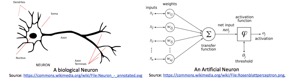
Artificial Neural Networks are inspired by Human Neural System. In the human neural system, axons of one neuron are connected with dendrites of another and they are regulating electric signals by using chemicals. This is the higher-level working of the human neurons. The number of these neurons is used for complex decision-making. It's just an intro 😃.
Logistic Regression
Problem
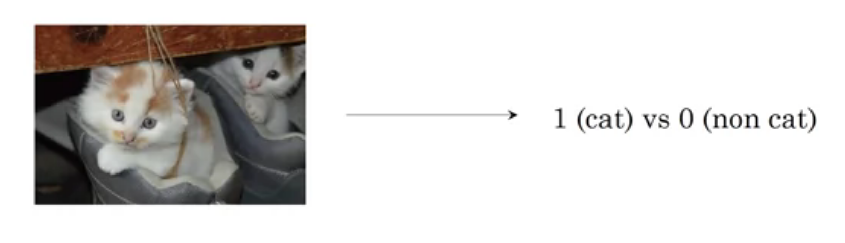
We have to find is there a cat in the image or not. This is binary classification because either cat is present or not in the image (1 or 0).
Before we start learning logistic regression, let's see how the image is stored and presented on a computer because we have to work on these images. Images are continuous signals in space but storing and processing continuous signals is too hard 🙁. So images are discretized and then stored and processed in computers. images are stored in a 3D matrix with 3 channels i.e. red, green, blue (RGB).
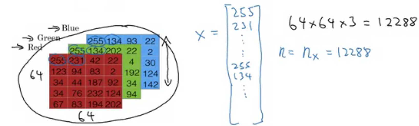
As shown in the above image, images are stored in a 3D matrix. But for training on logistic regression, we need vector as an input. So We will roll out this image into a long column vector. given image is 64x64x3 size where \(1^{st}\) 64 is height and \(2^{nd}\) width of the image. Actually, it depends on the situation. for example, in NumPy img.shape gives the first dimension as the height of the image while mentioning the resolution of the image, we do the opposite like 1920x1080.
So the problem: Given a cat picture \(X\), we want probability of cat in image i.e. \(\hat{y} = P(y=1|x)\).
Notation
We will see all notation in the basic neural networks. some of them are not used in logistic regression but we need them as we progress in the article.
Sizes
- \(m\): number of examples in dataset
- \(n_x\): input size
- \(n_y\): output size
- \(n^{[l]}_h\): Number of hidden units in \(l^{th}\) layer.
- \(L\): number of layers in network.
Objects
- \(X \in \mathbb{R}^{n_x \times m}\) is the input matrix
- \(x^i \in \mathbb{R}^{n_x}\) is the \(i^{th}\) example represented as a column vector
- \(Y \in \mathbb{R}^{n_y \times m}\) is the label matrix or actual output while training
- \(y^{(i)} \in \mathbb{R}^{n_y}\) is the output label for the \(i^{th}\) example
- \(W^{[l]} \in \mathbb{R}^{n^{[l]} \times n^{[l-1]}}\) is the weight matrix of \(l^{th}\) layer
- \(b^{[l]} \in \mathbb{R}^{number\space of\space units\space in\space next\space layer}\) is the bias vector in the \(l^{th}\) layer
- \(\hat{y} \in \mathbb{R}^{n_y}\) is the predicted output vector. Also denoted by \(a^{[L]}\).
Algorithm
Given \(X\), we want \(\hat{y} = P(y=1|0)\). As below image, we will give input as rolled image and output will be 1 if the cat in image else 0. in the image, \( w_1, w_2, ..., w_n \) are weights and \(b\) is the bias. These are learning parameters means we will learn them while the training phase.
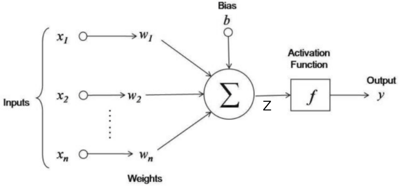
if we want to explain above image in one line then this line will be like this weighted sum over input is added to bias and whatever we got, pass it to activation function. Here weighted sum means multiply weights to respective input i.e. \(x_i * w_i\) and add them. Lets consider \(Z\) as a sum of weighted sum of input and bias.
\[
Z = b + \sum \limits_{i=1}^n x_i \times w_i
\]
Activation Function
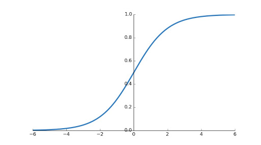
If you are familiar with linear regression then you might saw above image except activation function. In linear regression, we are finding real value i.e. \(Z\) but here we want probability of cat in image then it must be in \([0,1]\). And also it introduces non-linearity to the output \(Z\). We will use sigmoid activation function in this turtorial. There are other activations functions are also available like ReLU, Leaky ReLU, tanh etc.
\[
\sigma(Z) = \frac{1}{1+e^{-Z}}
\]
We need derivative of sigmoid function while sending error backward. So lets find now.
\[
\begin{align*}
\sigma'(Z) &= \frac{d}{dZ} . \frac{1}{1 + e^{-Z}} \\
&= \frac{d}{dZ}(1+e^{-Z})^{-1} \\
&= -(1+e^{-Z})^{-2}(-e^{-Z}) \\
&= \frac{e^{-Z}}{(1+e^{-Z})^2} \\
&= \frac{1}{1+e^{-Z}} (1+\frac{1}{1+e^{-Z}}) \\
&= \sigma(Z).(1-\sigma(Z))
\end{align*}
\]
When you plot sigmoid function, you will find graph shown below.
Training
Weights \(W^{[l]}\) are initialized randomly to eliminate symmetry problem which arises when we initialize weights to zeros. Biases can be initialized to zeros.
Basic steps are
1. Ininitialize weights and biases
2. forward pass means find \(\hat{y}\) using input and weights, biases
3. compare \(\hat{y}\) with \(Y\) i.e. predicted output with actual output and then backpropagate errors to make changes appropriately in weights and biases.
Lets take example. We have dataset with 10000 (\(m\)) images of with cat and without cat in it. when every image of size \(64 \times 64\times 3\) rolled out forms 12228 (\(n_x\)) features long vector. We got input \(X^{n_x \times m}\). Now label (Actual Output) for these examples is \(Y^{1 \times m}\).
Let's see code for initializing and forward pass.
import numpy as np

# suppose we have imput and output with us.
print(X.shape)  # (12228, 10000)
print(Y.shape)  # (1, 10000)

# initialize weights and biases
W = np.random.rand(12228, 1) # input * output
b = np.zeros(1,)

# learning rate
alpha = 0.001

# Now forward pass
Z = np.dot(W.T, X) + b

def sigmoid(X):
    return 1 / (1 + np.exp(- X))

def inv_sigmoid(X):
    return sigmoid(X) * (1-sigmoid(X))

y_hat = sigmoid(Z)Now time for Back Propagation. But it is too risky to say backpropagation because, in logistic regression, the error is not sent back to another layer (😃 Only a Single layer). For computing loss in a single training example, we will use binary cross-entropy loss and we can formulate the loss (error) function as
\[
L(\hat{y},y) = -(y\log({\hat{y}}) + (1-y)\log({1-\hat{y}}))
\]
We can also use our loss function used in linear regression \( L(\hat{y},y) = \frac{1}{2} (\hat{y} - y)^2\) but this loss function is non-convex So its too hard to find global minima.
Until now we defined loss function which can tell us that How good a particular example doing? But we want to find How good all examples doing?. For that purpose, we need cost function and it can be defined as
\[
J(W,b) = \frac{1}{m} \sum \limits_{i=1}^m L(\hat{y}^{i},y^{i})
\]
Gradient Descent
Now the only remaining job is to send loss backward and update weights and biases appropriately. For updating these parameters, we have to find cost w.r.t. weights and biases. Like below
\[
\begin{align*}
W &= W - \alpha * \frac{\partial{J}(W,b)}{\partial{W}} \\
b &= b - \alpha * \frac{\partial{J}(W,b)}{\partial{b}}
\end{align*}
\]
In the above equation, \(\alpha\) is the learning rate.
The amount that the weights are updated during training is referred to as the step size or the learning rate. Specifically, the learning rate is a configurable hyperparameter used in the training of neural networks that has a small positive value, often in the range between 0.0 and 1.0.
To find \(\frac{\partial{J}(W,b)}{\partial{W}}\) and \(\frac{\partial{J}(W,b)}{\partial{b}}\), we need to expand equation of \(J(W,b)\).
It's time to find gradients w.r.t. weights and biases. currently, call \(\hat{y}\) as \(a\). and for sake of simplicity, put \(\frac{1}{m}\) aside.
Now we will use above 2 equations to find \(\frac{\partial{J}(W,b)}{\partial{W}}\) and \(\frac{\partial{J}(W,b)}{\partial{b}}\)
\[
\begin{align*}
\frac{\partial{J}( W,b )}{\partial{W}} &= \frac{\partial{J}{(W,b)}}{\partial{Z}} \frac{\partial{Z}}{\partial{W}} \\
&=(\frac{1}{m})(a-y) . X^T \\
\frac{\partial{J}(W,b)}{\partial{b}} &= \frac{\partial{J}{(W,b)}}{\partial{Z}} \frac{\partial{Z}}{\partial{b}} \\
&=(\frac{1}{m})(a-y)
\end{align*}
\]
Finally done 😇. Time for code.
# Find cost
cost = -(1/m) * (Y*np.log(y_hat)+(1-Y)*np.log(1-y_hat))

dw = (1/m) * np.dot((y_hat - y), X.T)
db = (1/m)* np.sum(y_hat - y, axis=1, keeps_dim=True)

# update w and b
W = W - alpha * dw
b = b - alpha * dbNeural Network
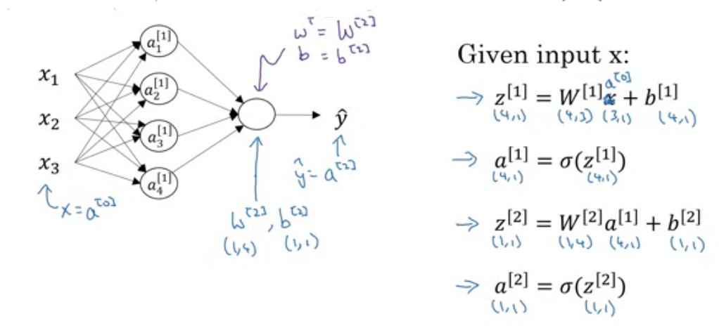
Still, now we learned logistic regression and updating parameters in it. A logistic regression unit is also called a neuron in a neural network. You can compare both neuron and neural networks in the below image. Neurons are stacked in 2-dimensional space and all neurons from the previous layer are connected to all neurons in the current layer.
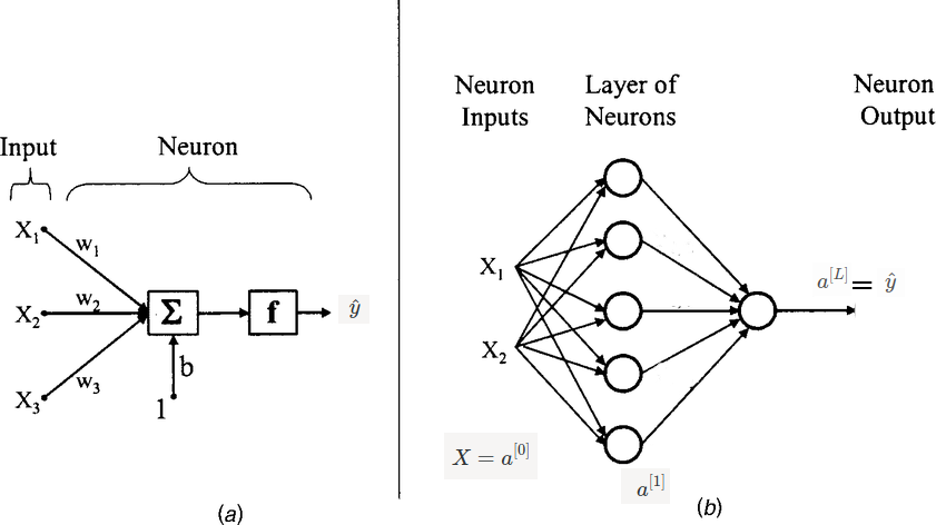
In the above image (b), 2 inputs are given to the Hidden layer and all 5 neurons in the hidden unit produce \(a^{[1]}\) which will pass to the output layer. In the image, 1 circle means 1 neuron. and (b) has 2 layers (Input is not considered as a layer). remember \(a^{[l]}_i\) means activations produced by \(i^{th}\) unit in \(l^{th}\) layer.
Forward Propagation
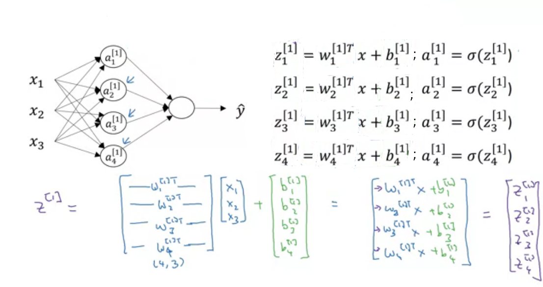
In the above image, \(x\) is our \(X\) in logistic regression. In logistic regression, we saw \(W\) is weight matrix but here we have a number of neurons so for each neuron we have a weight matrix and represented by \(W^{[l]}_i\) where \(l\) is layer and \(i\) is unit(neuron) in that layer. and also separate bias for each neuron \(b^{[l]}_i\). But while implementing, we use vectorization for fast computation. So all weights for neurons are stacked and created a row vector of \(W^{[l]}_i\) for each layer. Now weights of \(1^{st}\) layer are \(W^{[1]}\). Similarly, biases are also stacked and created column vectors.
Suppose, We are at layer \(l\) so previous layer \(l-1\) has \(n_{l-1}\) units and current layer \(l\) has \(n_{l}\) units then shape of weight matrix of layer \(l\) will be \(n_l \times n_{l-1}\). and shape of bias matrix will be \(n_l \times 1\). I know you are confused because shape of weight matrix in logistic regression is opposite what we are seeing here. To make implementation simple we are doing this. You can use another approach also.
Let's implement it in python as shown in the above image.
# We already have X and Y with us
# define units list
units = [3,4,1] # input, hidden, output

#initialise weights and biases
W_1 = np.random.rand(units[1],units[0])
b_1 = np.zeros((units[1],1))

W_2 = np.random.rand(units[2],units[1])
b_2 = np.zeros((units[2],1))

# Feed forward
z_1 = np.dot(W_1,X) + b_1
a_1 = sigmoid(z_1)

z_2 = np.dot(W_2,a_1) + b_2
y_hat = sigmoid(z_2) # or a_2
Back Propagation
We already saw in logistic regression that how to update \(W^{[2]}\) and \(b^{[2]}\) but for updating \(W^{[1]}\) and \(b^{[1]}\), we need \(\frac{\partial{J}(W,b)}{\partial{W^{[1]}}}\) and \(\frac{\partial{J}(W,b)}{\partial{b^{[1]}}}\); here \(W\) and \(b\) are considered as all weights and biases in network. means cost of final prediction. Lets find some more derivatives. But before that, see computation graph for our 2 layer neural network.
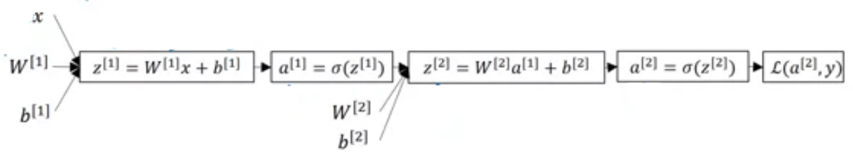
From the above graph, we can find the below equations. You may think that Why these equations re-arranged like that? Now, these equations can work with multiple examples at a time.
\[
\begin{align*}
\frac{\partial{J}(W,b)}{\partial{Z^{[1]}}} &= (\frac{\partial{Z^{[2]}}}{\partial{a^{[1]}}} . \frac{\partial{J}(W,b)}{\partial{Z^{[2]}}}) * \frac{\partial{a^{[1]}}}{\partial{Z^{[1]}}} \\
&= (W^{[2]T} . \frac{\partial{J}(W,b)}{\partial{Z^{[2]}}}) * \sigma'{(Z^{[1]})}\\
\end{align*}
\]
Now we can find \(\frac{\partial{J}(W,b)}{\partial{W^{[1]}}}\) and \(\frac{\partial{J}(W,b)}{\partial{b^{[1]}}}\)
\[
\begin{align*}
\frac{\partial{J}(W,b)}{\partial{W^{[1]}}} &= \frac{\partial{J}(W,b)}{\partial{Z^{[1]}}}.\frac{\partial{Z^{[1]}}}{\partial{W^{[1]}}} \\
&= \frac{\partial{J}(W,b)}{\partial{Z^{[1]}}}.X^{T} \\
\frac{\partial{J}(W,b)}{\partial{b^{[1]}}} &= \frac{\partial{J}(W,b)}{\partial{Z^{[1]}}}.\frac{\partial{Z^{[1]}}}{\partial{b^{[1]}}} \\
&= \frac{\partial{J}(W,b)}{\partial{Z^{[1]}}}
\end{align*}
\]
Finally done 😇. Time for code.
# Some code copied from logistic regression
# Find cost
cost = np.sum(-(1/m) * (Y*np.log(y_hat)+(1-Y)*np.log(1-y_hat)))

dZ_2 = np.array(y_hat - y)
dw2 = (1/m) * np.dot(dZ_2, a_1.T)
db2 = (1/m)* np.sum(dZ_2, axis=1, keepdims=True)

dZ_1 = np.dot(W_2.T,dZ_2) * inv_sigmoid(z_1)
dw1 = (1/m) * np.dot(dZ_1, a_1.T)
db1 = (1/m)* np.sum(dZ_1, axis=1, keepdims=True)

# Update weights
W_1 = W_1 - alpha * dw1
b_1 = b_1 - alpha * db1

W_2 = W_2 - alpha * dw2
b_2 = b_2 - alpha * db2