Deep Neural Network with MNIST Digit Recognition Example from Scratch

This will be the $3^{rd}$ and last article in neural network and deep learning the series. We will see multiclass classification in this article. Before that, check previous articles first and return to these articles. Below are the links to these previous articles.

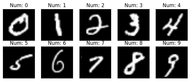
Still now we only saw binary classification problems (either 1 or 0). In this article, We will see multiclass (means one of the many classes) problem. Let's see directly what is MNIST handwritten digit dataset is. It contains 60000 images of handwritten digits (0-9). Total 10 classes 🙄 i.e. multiclass classification. all images are grayscale and 28x28 in size. You can check some samples in the below image.

Before that take simple network with multiclass output. 4 class neural network is shown in below image. Here, shape of $\hat{y}$ will be (4, m) where m is number of examples. Generally shape of $\hat{y}$ is (K, m) where K is number of classes.

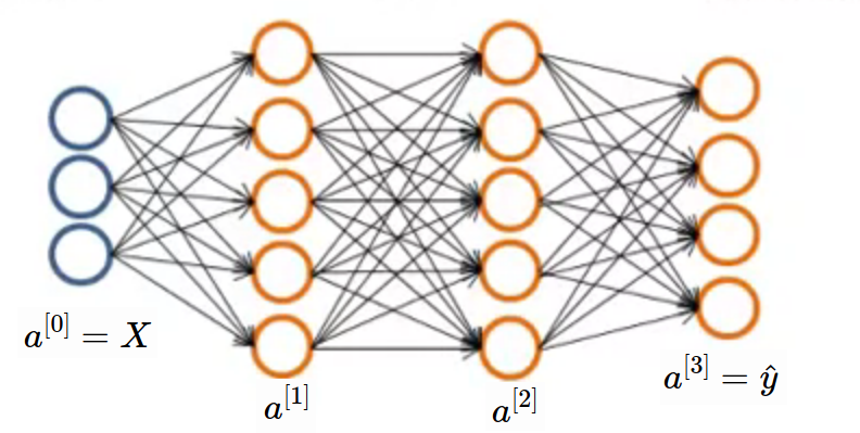
Lets revise some terminologies. $m$ will be number of samples in dataset and $n_x$ will be size of input then $(n_x, m)$ will be the input matrix size. And $n_y = K$ will be output size then $(n_y, m)$ will be the output matrix size. As per our above neural network, label will be one of the following column vector because only 1 out of 4 class will be present for a sample in our example. for our convenience, suppose cat, dog, frog and rabbit these are the classes. So $\begin{bmatrix} 1\ 0\ 0\ 0\ \end{bmatrix}$ is the cat class. This kind of encoding is called as One Hot Encoding because for some particular sample only one value is hot (1) and other are cool (0).

$$ Y \in \begin{bmatrix} 1 \\ 0 \\ 0 \\ 0 \end{bmatrix}, \begin{bmatrix} 0 \\ 1 \\ 0 \\ 0 \end{bmatrix}, \begin{bmatrix} 0 \\ 0 \\ 1 \\ 0 \end{bmatrix}, \begin{bmatrix} 0 \\ 0 \\ 0 \\ 1 \end{bmatrix} $$

Initialize Variables

In general, our data will look like the following matrices. $X$ is input and $Y$ is output. in below equation, $K$ is number of classes and we use $K$ and $n_y$ interchangebly.

$$ X = \begin{bmatrix} x_{11} & x_{21} & \dots & x_{m1}\\ \vdots & \vdots & \dots & \vdots\\ x_{1n_x} & x_{2n_x} & \dots & x_{mn_x} \end{bmatrix} ; Y = \begin{bmatrix} y_{11} & y_{21} & \dots & y_{m1}\\ \vdots & \vdots & \dots & \vdots\\ y_{1K} & y_{2K} & \dots & y_{mK} \end{bmatrix} $$

Before we jump into forward pass, lets create dataset. We will create random data and at last check whether cost is decreasing or not. If cost is decreasing after each epoch then we can say that our model is working fine.

import numpy as np

# set seed
np.random.seed(95)

# number of examples in dataset
m = 6
# number of classes
K = 4
# input shape
n_x = 3

# input (n_x, m)
X = np.random.rand(n_x, m)

# hypothetical random labels
labels = np.random.randint(K, size=m)

# convert to one hot encoded
Y = np.zeros((4,6))
for i in range(m):
  Y[labels[i]][i] = 1

print("X", X)
print("Labels",labels)
print("Y",Y)

Output

X:
 [[0.22880349 0.19068802 0.88635967 0.7189259  0.53298338 0.8694621 ]
 [0.72423768 0.48208699 0.7560772  0.97473999 0.5083671  0.95849135]
 [0.49426336 0.51716733 0.34406231 0.96975023 0.25608847 0.40327522]]
Labels:  [2 1 3 0 0 3]
Y:
 [[0. 0. 0. 1. 1. 0.]
 [0. 1. 0. 0. 0. 0.]
 [1. 0. 0. 0. 0. 0.]
 [0. 0. 1. 0. 0. 1.]]

Now time to randomly intialize weights and biases to 0. We will create units list which tells us, How may neurons in each layers?

# units in each layer
# first number (3) is input dimension
units = [3, 5, 5, 4]

# Total layers except input
L = len(units) - 1

# parameter dictionary
parameters = dict()

for layer in range(1, L+1):
    parameters['W' + str(layer)] =   np.random.rand(units[layer],units[layer-1])
    parameters['b' + str(layer)] = np.zeros((units[layer],1))

Forward Pass

We saw in forward pass in previous article and no change is required for feed forward. So let's copy equations from previous article. Normally people uses Softmax activation function at last layer but for simplicity, we will continue using Sigmoid.

\[
\begin{align*}
Z^{[l]} &= W^{[l]}.a^{[l-1]} + b^{[l]} \\
a^{[l]} &= g^{[l]}{(Z^{[l]})}
\end{align*}
\]

Lets write code for forward pass in python. We will use our generic code from previous article.

cache = dict()
cache['a0'] = X

for layer in range(1, L+1):
    cache['Z' + str(layer)] = np.dot(parameters['W' + str(layer)],cache['a' + str(layer-1)]) 
    						+ parameters['b' + str(layer)]
    cache['a' + str(layer)] = sigmoid(cache['Z' + str(layer)])

Backward Pass

Still what we saw is from previous article. Now the most important part i.e. Loss Function & Cost Function. We already saw difference between loss function and cost function in article 1 of this series. We will use Binary Cross Entropy generalized for $K$ classes as our loss function. The formula for it is same as Binary Cross Entropy extended for multiple classes. Below, second equation is vectorized version of first equation.

$$ \begin{align*} L(\hat{y},y) &= - \frac{1}{K} \sum \limits_{i=1}^K [y_i\log{\hat{(y_i)}} + (1-y_i)\log{(1-\hat{y_i})}] \\ &= - [y\log{\hat{(y)}} + (1-y)\log{(1-\hat{y})}] \end{align*} $$

So the cost function will be the addition of all losses over all examples. So cost function will be

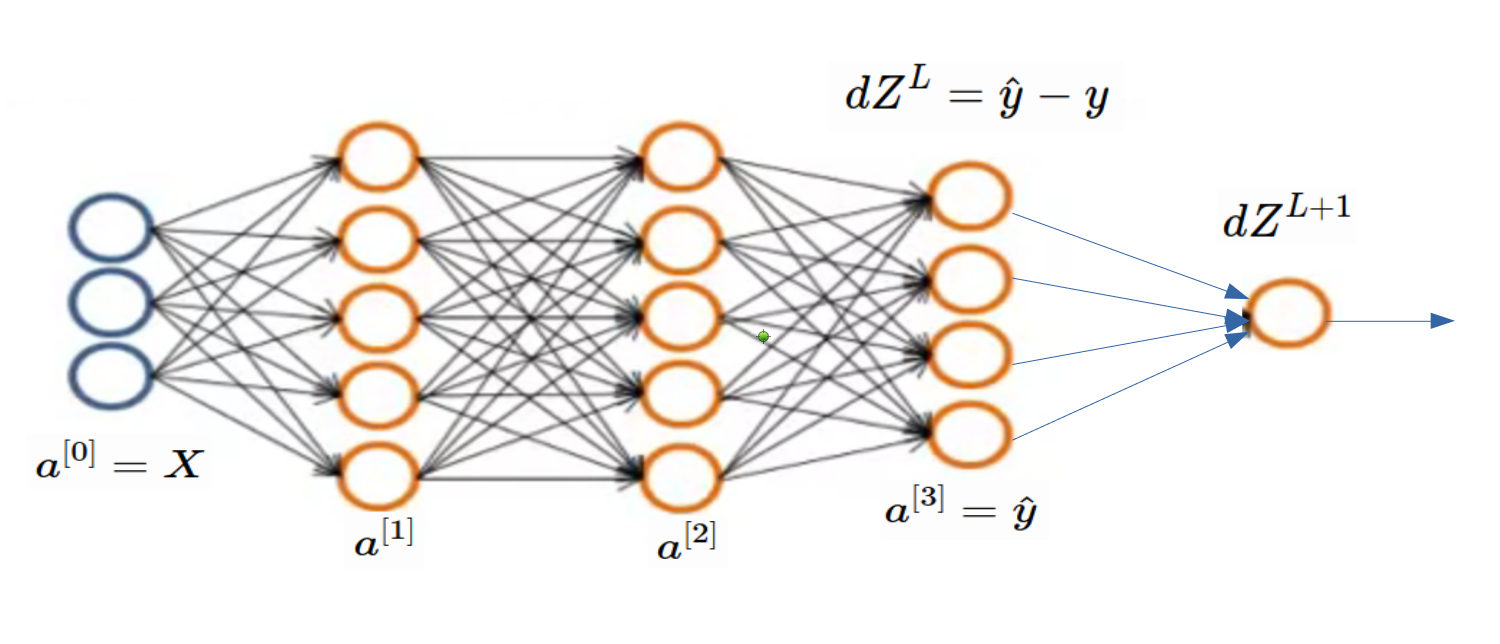
$$ \begin{align*} J(W,b) &= \frac{1}{m} \sum \limits_{i=1}^m L(\hat{y}^{i},y^{i}) \\ &= - \frac{1}{K} \frac{1}{m} \sum \limits_{j=1}^m \sum \limits_{i=1}^K [y_i^j\log{\hat{(y_i^j)}} + (1-y_i^j)\log{(1-\hat{y_i^j})}] \\ &= - \frac{1}{m} \sum \limits_{j=1}^m [y^j\log{\hat{(y^j)}} + (1-y^j)\log{(1-\hat{y^j})}] \end{align*} $$

Now its time of finding derivative of loss function. Before that check below image so that you can compare binary classification problem with multiclass classification. When we find $dZ^L$, we are done. As per below image, finding $dZ^L$ is tricky part and all gradient in layers before it can be found using our regular (generic) code. Check previous article.

In below equations, $W$ & $b$ are representing all weights and biases of network.

$$ \begin{align*} dZ^L &= \frac{\partial{J(W,b)}}{\partial{Z^L}} \\ &= \frac{\partial}{\partial{Z^L}}[- \frac{1}{m} \sum \limits_{j=1}^m [y^j\log{\hat{(y^j)}} + (1-y^j)\log{(1-\hat{y^j})}]] \\ &= - \frac{1}{m} \sum \limits_{j=1}^m [\frac{\partial}{\partial{Z^L}} [y^j\log{\hat{(y^j)}} + (1-y^j)\log{(1-\hat{y^j})}]] \\ &=- \frac{1}{m} \sum \limits_{j=1}^m (y^i - \hat{y^i}) \\ &= \frac{1}{m} \sum \limits_{j=1}^m ( \hat{y^i} - y^i) \end{align*} $$

Above equation can further vectorized for speedup. I will start another series on High Performance Computing as early as possible. In that article, we will see advantages of vectorization.

\[
\begin{align*}
dZ^L &= \frac{1}{m} (\hat{y}-y)
\end{align*}
\]

Its code time 😇. Let's implement backpropagation. You may say that both codes from previous article and this article are same. it's because vectorized equation for $dZ^L$ is same for both binary classification and multiclass classification. Remember our example with random data doesn't make any sense because it don't have any pattern. We care about cost is decreasing or not?. You can find colab notebook in references and code section. Just care about cost decreasing or not.

def cost(y,y_hat):
  return -np.sum(y*np.log(y_hat) + (1-y)*(np.log(1-y_hat)))

y_hat = cache['a' + str(L)]
cost_ = cost(y,y_hat)
cache['dZ' + str(L)] = (1/m) * (y_hat - Y)
cache['dW' + str(L)] = np.dot(cache['dZ' + str(L)], cache['a' + str(L-1)].T)
cache['db' + str(L)] = np.sum(cache['dZ' + str(L)], axis=1, keepdims=True)

for layer in range(L-1,0,-1):
  cache['dZ' + str(layer)] = np.dot(parameters['W' + str(layer+1)].T, cache['dZ' + str(layer+1)]) 
  							* inv_sigmoid(cache['Z' + str(layer)])
  cache['dW' + str(layer)] = np.dot(cache['dZ' + str(layer)], cache['a' + str(layer-1)].T)
  cache['db' + str(layer)] = np.sum(cache['dZ' + str(layer)], axis=1, keepdims=True)

MNIST Handwritten Digit Recognition

In above random data example, data and output doesn't make any sense so we will see real life example of handwritten digit classification. You already saw about dataset at start of this article.

Load Dataset

Now we will load data. Link to dataset is also given in references and code section.

import numpy as np
np.random.seed(95)

# Load CSV File
data = np.genfromtxt("mnist_train.csv",delimiter = ',')

# first column is labels
y = data[:,0]

# rest 784 columns are features / pixel values.
X = data[:,1:785].T

# Some constants
K = 10  # No of classes
alpha = 0.1  # Learning rate
m = 60000  # No of examples

# convert to one hot encoded
Y = np.zeros((K,m))
for i in range(m):
  Y[int(y[i]),i] = 1

# print shape of input and output/label
print('Shape of X:',X.shape)
print('Shape of y:',y.shape)
print('Shape of Y:',Y.shape)

Output

Shape of X: (784, 60000)
Shape of y: (60000,)
Shape of Y: (10, 60000)

Initialize Weights and Biases

# units in each layer
# first number (784) is input dimension
units = [784, 128, 64, 10]

# Total layers
L = len(units) - 1

# parameter dictionary
parameters = dict()

for layer in range(1, L+1):
    parameters['W' + str(layer)] = np.random.normal(0,1,(units[layer],units[layer-1]))
    parameters['b' + str(layer)] = np.zeros((units[layer],1))

Define Sigmoid and Derivative of Sigmoid Function

def sigmoid(X):
    return 1 / (1 + np.exp(- X))

def inv_sigmoid(X):
    return sigmoid(X) * (1-sigmoid(X))

Forward Pass

cache = dict()
def forward_pass(X):
  cache['a0'] = X

  for layer in range(1, L+1):
    cache['Z' + str(layer)] = np.dot(parameters['W' + str(layer)],cache['a' + str(layer-1)]) + parameters['b' + str(layer)]
    cache['a' + str(layer)] = sigmoid(cache['Z' + str(layer)])

Backward Pass

We will use batch size of 10 samples because of that you will find $\frac{1}{10}$ instead of $\frac{1}{m}$ (All data at a time).

def cost(y,y_hat):
  return -np.sum(y*np.log(y_hat) + (1-y)*(np.log(1-y_hat)))

def back_prop(Y):
  y_hat = cache['a' + str(L)]
  cache['dZ' + str(L)] = (1/10)*(y_hat - Y)
  cache['dW' + str(L)] = np.dot(cache['dZ' + str(L)], cache['a' + str(L-1)].T)
  cache['db' + str(L)] = np.sum(cache['dZ' + str(L)], axis=1, keepdims=True)

  for layer in range(L-1,0,-1):
    cache['dZ' + str(layer)] = np.dot(parameters['W' + str(layer+1)].T, cache['dZ' + str(layer+1)]) * inv_sigmoid(cache['Z' + str(layer)])
    cache['dW' + str(layer)] = np.dot(cache['dZ' + str(layer)], cache['a' + str(layer-1)].T)
    cache['db' + str(layer)] = np.sum(cache['dZ' + str(layer)], axis=1, keepdims=True)

Update Weights and Biases

def update_weights():
  for layer in range(1, L+1):
    parameters['W' + str(layer)] = parameters['W' + str(layer)] - alpha * cache['dW' + str(layer)]
    parameters['b' + str(layer)] = parameters['b' + str(layer)] - alpha * cache['db' + str(layer)]

Start Training

epoch = 30

for i in range(epoch):
  cost_tot = 0
  for j in range(6000):
    forward_pass(X[:,j*10:j*10+10])
    cost_tot += cost(Y[:,j*10:j*10+10],cache['a' + str(L)])
    back_prop(Y[:,j*10:j*10+10])
    update_weights()
  if i%5 == 0:
    print('epoch ',i,' ',cost_tot)

Output

epoch  0   119429.14804683565
epoch  5   102128.37509302271
epoch  10   90151.75500527128
epoch  15   86009.41961305328
epoch  20   88218.24177992699
epoch  25   90432.20939203199
epoch  30   92974.92502732007
epoch  35   93986.34837736617
epoch  40   92380.93127681084
epoch  45   90417.26686598927
epoch  50   101933.2601655828

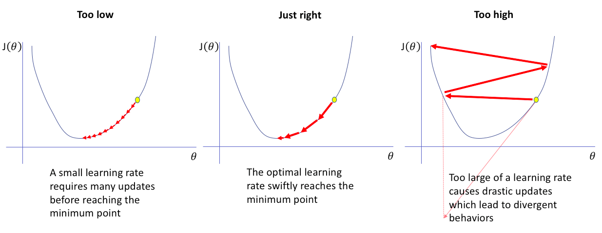
Above output shows, cost is decrasing still $45^{th}$ epoch but for $50^{th}$ epoch, it is increased. Reason of this is Learning Rate. If learning rate is too small, training takes more time and if learning rate is too high then what happens you already experienced. Finding not too high, not too low learning rate is difficult problem for particular application. We will see another article with heading Hyper parameter tunning tricks in near future.

Check Some Samples

forward_pass(X[:,0:10])

# axis 0 means max columnwise
# axis 1 means max rowwise
predicted = cache['a3'].argmax(axis=0)
actual = Y[:,:10].argmax(axis=0)

print('Actual Labels: ', actual)
print('Predicted Labels: ',predicted)

Output

Actual Labels:  [5 0 4 1 9 2 1 3 1 4]
Predicted Labels:  [3 0 4 1 4 6 1 3 1 4]

References and Code

[1] Dataset : handwritten digit recognition

You can find code (MNIST)

You can find code (Random Data)

Initialize Variables

Forward Pass

Backward Pass

MNIST Handwritten Digit Recognition

Load Dataset

Initialize Weights and Biases

Define Sigmoid and Derivative of Sigmoid Function

Forward Pass

Backward Pass

Update Weights and Biases

Start Training

Check Some Samples

References and Code

You might also like...